Projection Images
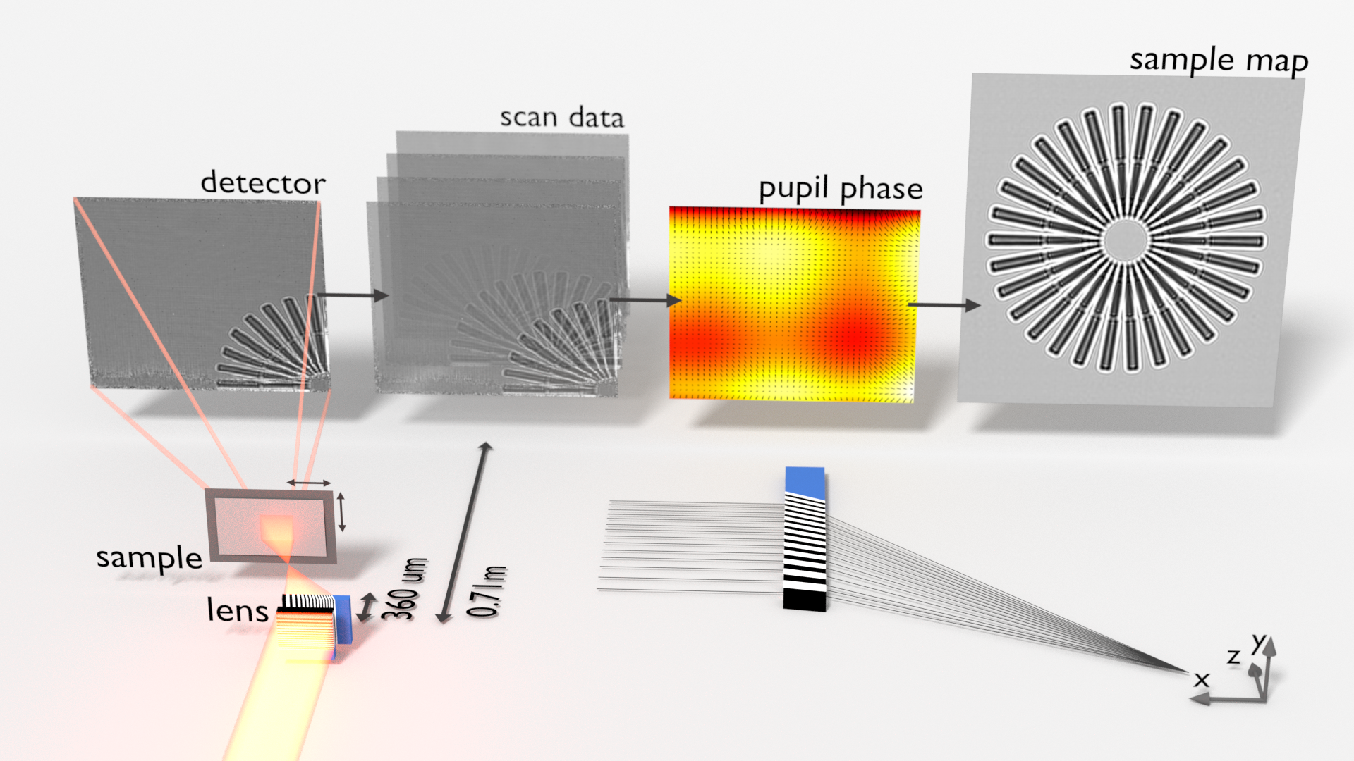
Here we describe a projection image, formed by shining potentially aberrated focused monochromatic light through a thin sample onto a detector far from the focus, as a distorted view of a magnified image one would have seen with plane wave illumination and the detector placed close to the sample.
OK, that’s a lot of words. But basically we are drawing the connection between the images formed by:
so that we can determine the lens aberrations and form an un-distorted view of the sample projection image.
Magnified Aberrated Projection Images
Say that the light wavefronts at the plane of the sample and detector are given by:
\[\begin{split}\begin{align}
P(\mathbf{x}, z_1) &= a(\mathbf{x}) e^{i\phi(\mathbf{x})} && \text{sample plane} \\
P(\mathbf{x}, z_2) &= A(\mathbf{x}) e^{i\Phi(\mathbf{x})} && \text{detector plane}
\end{align}\end{split}\]
where \(z_1\) and \(z_2\) are the focus to sample and sample to detector distances respectively, \(\phi\) and \(\Phi\) are the respective wavefront phases and \(a\) and \(A\) are the wavefront amplitudes, we’ll call \(A\) the aperture function and \(P(x, z_2)\) the pupil function.
Now we put a thin sample, with a transmission function \(T\), into the beam of light a distance \(z_1\) from the focal point. Then the image formed on the detector is given by the mod square of the Fresnel integral:
\[\begin{align}
I^{z_1}_\phi(\mathbf{x}, z_2) &= \big| \left[ T(\mathbf{x}) P(\mathbf{x}, z_1)\right] \otimes e^{i\pi \frac{\mathbf{x}^2}{\lambda z_2}} \big|^2
\end{align}\]
On the other hand, if we had un-abberrated plane wave illumination shinning through the sample onto a detector placed at a distance \(z_\text{eff}\) from the sample then we would see
\[\begin{split}\begin{align}
I^{\infty}_0(\mathbf{x}, z_\text{eff}) &= \big| T(\mathbf{x}) \otimes e^{i\pi \frac{\mathbf{x}^2}{\lambda z_\text{eff}}} \big|^2 \\
\end{align}\end{split}\]
It turns out that \(I^{z_1}_\phi\) is, more or less, a magnified view of \(I^{\infty}_0\) with geometric distortions caused by the phase aberrations:
\[\begin{split}\begin{align}
I^{z_1}_\phi(\mathbf{x}, z_2) &\approx
A^{2}(\mathbf{x}) I^{\infty}_0(\mathbf{x}
- \frac{\lambda z_\text{eff}}{2\pi} \nabla\phi(\mathbf{x}), z_\text{eff}) \quad \text{and} \\
I^{\infty}_0(\mathbf{x}, z_\text{eff}) &\approx
A^{-2}(\mathbf{x}) I^{z_1}_\phi(\mathbf{x}
- \frac{\lambda z^-_\text{eff}}{2\pi} \nabla\Phi(\mathbf{x}), z_2) \quad \text{where} \\
M = \frac{z_1 + z_2}{z_1} \quad \text{and}
\quad z_\text{eff} &= \frac{z_2}{1 + \frac{\lambda z_2}{2 \pi} \frac{1}{2}\langle\nabla^2 \phi\rangle_{\mathbf{x}}} \quad \text{and}
\quad z^-_\text{eff} = \frac{-z_2}{1 + \frac{\lambda (-z_2)}{2 \pi} \frac{1}{2}\langle\nabla^2 \Phi\rangle_{\mathbf{x}}}
\end{align}\end{split}\]
Fresnel Scaling Theorem
- The above equation is a more general form of the Fresnel scaling theorem, which states that:
The projected image of a thin scattering object from a point source of monochromatic light is equivalent to a magnified defocused image of the object formed by moving the point source of light infinitely far away.
and we can see that this is indeed the case if we set \(\Phi = \pi \mathbf{x}^2 / \lambda (z_1+z_2)\) and \(A=M^{-2}\) in the above equation. So we have:
\[\begin{align}
\Phi(\mathbf{x}) &= \frac{\pi \mathbf{x}^2}{\lambda (z_1 + z_2)} \quad
\nabla \Phi(\mathbf{x}) = \frac{2\pi \mathbf{x}}{\lambda (z_1 + z_2)} \quad
\frac{1}{2}\nabla^2 \Phi(\mathbf{x}) = \frac{2\pi}{\lambda (z_1 + z_2)}
\end{align}\]
and:
\[\begin{split}\begin{align}
z^-_\text{eff} &= \frac{z_2}{\frac{\lambda z_2}{2 \pi} \langle\nabla^2 \Phi\rangle_{\mathbf{x}}-1}
= \frac{z_2}{\frac{\lambda z_2}{2 \pi} \frac{2\pi}{\lambda (z_1 + z_2)} -1}
= -\frac{z_2}{z_1}(z_1+z_2) \\
\end{align}\end{split}\]
and:
\[\begin{split}\begin{align}
\mathbf{x} - \frac{\lambda z_\text{eff}}{2\pi} \nabla\Phi(\mathbf{x}) &= \mathbf{x} + \frac{\lambda }{2\pi}\frac{z_2}{z_1}(z_1+z_2) \frac{2\pi \mathbf{x}}{\lambda (z_1 + z_2)}
= \mathbf{x}\frac{z_1 + z_2}{z_1}
= M \mathbf{x} \\
\end{align}\end{split}\]
and finally:
\[\begin{align}
I^{\infty}_0(\mathbf{x}, z_\text{eff}) &\approx M^{-2} I^{z_1}_\Phi(M\mathbf{x}, z_2) \quad \text{as required}
\end{align}\]
Reciprocity of sample / detector phase
The two speckle-tracking formula imply the reciprocal relations:
\[\begin{align}
\frac{\lambda z^-_\text{eff}}{2\pi} \nabla\Phi(\mathbf{x}) &= -\frac{\lambda z_\text{eff}}{2\pi} \nabla\phi( \mathbf{x} - \frac{\lambda z^-_\text{eff}}{2\pi} \nabla\Phi(\mathbf{x}))
\end{align}\]
which relates the phase of the illumination wavefronts in the sample and detector planes respectively.
We can check this with a well known case, that of a point source of illumination with no aberrations. In this case:
\[\begin{split}\begin{align}
\nabla \phi(\mathbf{x}) = \frac{2\pi \mathbf{x}}{\lambda z_1} \quad
\nabla \Phi(\mathbf{x}) = \frac{2\pi \mathbf{x}}{\lambda (z_1 + z_2)} \\
\end{align}\end{split}\]
and therefore:
\[\begin{align}
z_\text{eff} = \frac{z_1 z_2}{z_1+z_2} \quad
z^-_\text{eff} = -\frac{z_2}{z_1}(z_1+z_2)
\end{align}\]
Let’s evaluate the left and right hand sides of the reciprocal formula:
\[\begin{split}\begin{align}
\text{LHS} &= -\frac{\lambda }{2\pi}\frac{z_2}{z_1}(z_1+z_2) \frac{2\pi \mathbf{x}}{\lambda (z_1+z_2)}
= -\frac{z_2}{z_1} \mathbf{x} \\
\end{align}\end{split}\]
and the RHS:
\[\begin{split}\begin{align}
\text{RHS} &= -\frac{\lambda }{2\pi}\frac{z_1 z_2}{z_1+z_2} \frac{2\pi}{\lambda z_1}( \mathbf{x} - \frac{\lambda z^-_\text{eff}}{2\pi} \nabla\Phi(\mathbf{x})) \\
&= -\frac{z_2}{z_1+z_2}( \mathbf{x} + \frac{\lambda}{2\pi} \frac{z_2}{z_1}(z_1+z_2)\frac{2\pi \mathbf{x}}{\lambda (z_1 + z_2)}) \\
&= -\frac{z_2}{z_1+z_2} \mathbf{x} \frac{z_1 + z_2}{z_1} \\
&= -\frac{z_2}{z_1}\mathbf{x} \quad \text{= LHS as required}
\end{align}\end{split}\]