Thon Rings

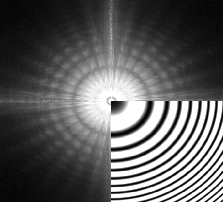
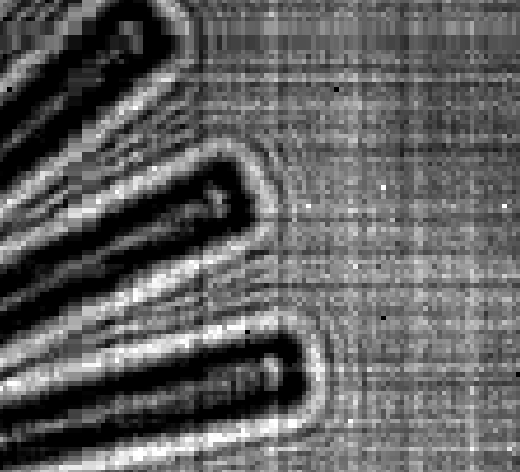
If you look at the defocused image of a thin sample with phase contrast, then you will see Fresnel fringes around the edges. See, for example, this image from the Siemens Star tutorial:

These fringes arise from the effective contrast transfer function, or optical transfer function, of the imaging system:

\[\begin{align} I(\mathbf{x}) &= \big| T(\mathbf{x}) \otimes \mathcal{F}^{-1}[\text{TF}](\mathbf{x}) \big|^2 \end{align}\]

where I is the image on a detector, T the transmission function of an object and TF is the transfer function of the imaging system.

For example, take free-space propagation:

\[\begin{align} I(\mathbf{x}) &= \big| T(\mathbf{x}) \otimes \mathcal{F}^{-1}[e^{-i\pi\lambda z_2\mathbf{q}^2}] \big|^2 \end{align}\]

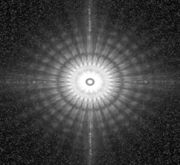
this roughly corresponds to the situation in the image above. Now if we take the Fourier transform of this image (see the image below) then we can often observe concentric rings modulating a complicated pattern. These are the Thon rings and they can be used to roughly estimate the TF, for example this might give us the propagation distance \(z_2\) in the above example.

Thin weakly scattering object

For a thin weakly scattering object we can approximate:

\[\begin{split}\begin{align} T(\mathbf{x}) &\approx e^{-i\frac{2\pi}{\lambda} \int dz n(\mathbf{x})} &&\text{projection approximation (thin sample)} \\ &&& \text{with refractive index } n(\mathbf{x}) = \delta_\lambda(\mathbf{x}) -i\beta_\lambda(\mathbf{x}) \\ &\approx e^{-\frac{2\pi}{\lambda} t(\mathbf{x}) (i\delta_\lambda + \beta_\lambda)} &&\text{single material of projected thickness } t(\mathbf{x}) \\ &\approx 1 - \frac{2\pi}{\lambda} t(\mathbf{x}) (\beta_\lambda + i \delta_\lambda) &&\text{weakly scattering} \end{align}\end{split}\]

Now we can approximate the Fourier transform of the image as:

\[\begin{align} \hat{I}(\mathbf{q}) &\approx \frac{2\pi}{\lambda}\hat{t}(q)\left[ i\delta_\lambda \left( \text{TF}^*(-\mathbf{q}) - \text{TF}(\mathbf{q}) \right) -\beta_\lambda \left( \text{TF}^*(-\mathbf{q}) + \text{TF}(\mathbf{q}) \right) \right] \quad \text{for } \mathbf{q} \neq 0 \end{align}\]

Pure phase contrast image

Let us consider the case of free-space propagation, and a pure phase contrast image (\(\beta_\lambda = 0\)):

\[\begin{split}\begin{align} \text{TF}(\mathbf{q}) &= e^{-i\pi\lambda z_2 \mathbf{q}^2} && \text{TF}^*(-\mathbf{q}) - \text{TF}(\mathbf{q}) = 2i\sin(\pi\lambda z_2 \mathbf{q}^2) \\ \hat{I}(\mathbf{q}) &= -\frac{4\pi}{\lambda} \delta_\lambda \hat{t}(\mathbf{q}) \sin(\pi\lambda z_2 \mathbf{q}^2) && \text{for } \mathbf{q} \neq 0 \end{align}\end{split}\]

The above image was actually made from:

\[\begin{align} \text{image}(q) &= \sum_n \big|\mathcal{F}[M(r) e^{-r^2 / 2 \sigma^2} I_n(r) / W(r) ](q) \big|^2 \end{align}\]

where \(n\) is the image number, \(M(r)\) is the mask, \(W(r)\) is the whitefield, and the Gaussian is applied to avoid Fourier aliasing artefacts. The image was then taken to the power of 0.1 to enhance the contrast.

Projection images

For projection imaging we have the approximation:

\[\begin{split}\begin{align} I^{z_1}_\phi(\mathbf{x}, z) &\approx \big|T(\mathbf{x}) \otimes e^{\frac{i \pi}{\lambda z^x_\Phi} \left( x - \frac{\lambda z}{2\pi} \Phi_{,x}(\mathbf{x})\right)^2 + \frac{i \pi}{\lambda z^y_\Phi} \left( x - \frac{\lambda z}{2\pi} \Phi_{,y}(\mathbf{x})\right)^2} \big|^2, \\ \text{where, } z^x_\Phi &= z \left(1 - \frac{\lambda z}{2\pi} \langle \Phi_{,xx} \rangle_x \right) \end{align}\end{split}\]

Here \(\Phi(\mathbf{x})\) is the phase profile of the probe in the plane of the detector. Now let us make a low order approximation for \(\Phi(\mathbf{x})\):

\[\begin{align} \Phi(\mathbf{x}) &= \frac{\pi x^2}{\lambda (z+z_x)} + \frac{\pi y^2}{\lambda (z+z_y)} \end{align}\]

Now we can take the Fourier transform and evaluate the effective transfer function of the imaging system:

\[\begin{split}\begin{align} \text{TF}(\mathbf{q}) &= e^{-i\pi \lambda z q^2} e^{-i\pi \lambda z^2 \left(\frac{q_x^2}{z_x} + \frac{q_y^2}{z_y}\right)}\\ &= e^{-i\pi \lambda z \left((1+\frac{z}{z_x})q_x^2 + (1+\frac{z}{z_y})q_y^2\right)} \end{align}\end{split}\]

OK, so what do our Thon rings look like?

\[\begin{split}\begin{align} \text{TF}^*(-\mathbf{q}) - \text{TF}(\mathbf{q}) &= 2i\sin(\pi \lambda z q'^2) \\ \text{TF}^*(-\mathbf{q}) + \text{TF}(\mathbf{q}) &= 2\cos(\pi \lambda z q'^2) \\ q'^2 &= (1+\frac{z}{z_x})q_x^2 + (1+\frac{z}{z_y})q_y^2 \end{align}\end{split}\]

and therefore

\[\begin{split}\begin{align} \hat{I}(\mathbf{q}) &\approx -\frac{4\pi}{\lambda}\hat{t}(q)\left[ \delta_\lambda \sin(\pi \lambda z q'^2) +\beta_\lambda \cos(\pi \lambda z q'^2) \right] \quad \text{for } \mathbf{q} \neq 0 \text{, and} \\ \big| \hat{I}(\mathbf{q}) \big|^2 &\approx \frac{8\pi^2}{\lambda^2}|\hat{t}(q)|^2\left[ \delta_\lambda \sin(\pi \lambda z q'^2) +\beta_\lambda \cos(\pi \lambda z q'^2) \right]^2 \quad \text{for } \mathbf{q} \neq 0 \end{align}\end{split}\]

it makes sence that, appart from \(\hat{t}(q)\), \(\hat{I}(\textbf{q})\) is real valued since TF is centrosymmetric.

Fitting

Let’s ignore the physics for a moment and say that we have some array \(I_{nm}\) given by:

\[\begin{align} I_{nm} &= \big| \hat{I}(\mathbf{q}_{nm})\big|^2 \end{align}\]

Now we filter the image, in order to flatten the contrast. Then we solve the problem:

\[\begin{align} I_{nm'} &= f_\sqrt{n^2 + m'^2} \quad \text{where} \quad m'= \text{scale_fs} \times m \end{align}\]

meaning that we are looking for the scaling factor along the fast scan axis of the array that makes the image most circular. Now we fit a and b in the following profile:

\[\begin{align} f_n &= (\sin(c n^2) + d\cos(c n^2))^2 \end{align}\]

Now we return to the physics: given scale_fs, c and d we would like to determine:

\[\begin{split}\begin{align} &z, z_x, z_y \quad \text{where}\\ &z = \text{sample to detector distance and} \\ &z_x, z_y = \text{are the x and y focus to sample distances} \end{align}\end{split}\]

With the results in the above sections we have that:

\[\begin{split}\begin{align} \text{scale_fs} &= \sqrt{\frac{1+z/z_x}{1+z/z_y}} \times \frac{N \Delta u_y}{M \Delta u_x} && \\ c &= \frac{\pi \lambda z}{(N\Delta u_y)^2} \left(1 + \frac{z}{z_y}\right) & d &= \frac{\beta_\lambda}{\delta_\lambda} \\ z_t &= z + \frac{1}{2}(z_x + z_y) && \end{align}\end{split}\]

where \(z_t\) is the (average) focus to detector distance, \(\Delta u_x\) and \(\Delta u_y\) are the pixel dimensions along x and y respectively, N and M are the number of pixels along the slow and fast scan axes and it is assumed that x is parallel to the fast scan axis and y is parallel to the slow scan axis.

So we have:

\[\begin{split}\begin{align} \delta z &= \frac{- a \pm \sqrt{a^2 + z_t^2(a/b-1)^2}}{a/b-1} & z_1 &= \frac{\delta z(a-b) + 2 z_t^2}{a+b+2z_t} \text{ where} \\ z_x &= z_1 - \delta z & z_y &= z_1 + \delta z \;,\\ a &= \frac{c (\text{scale_fs}M\Delta u_x)^2}{\pi \lambda} & b &= \frac{ c (N\Delta u_y)^2}{\pi \lambda} \;,\\ \end{align}\end{split}\]

and \(\delta z>0\) if \(\text{scale_fs} \times M \Delta u_x / (N \Delta u_y) > 1\).